Understanding Financial Time Series Models (Part I): ARMA and Market Dynamics

Chen Quant Academy Series -- Introducing Quantitative Models in Finance

Introduction: Is the Market Completely Random?

One of the first questions in quantitative finance is whether financial markets are entirely random or whether traces of the past continue to influence the future.

Figure 1 Time Series

At first glance, daily price movements appear chaotic. News arrives unexpectedly, investor sentiment changes rapidly, and external shocks constantly reshape expectations. On the other hand, we often hear expressions such as "the trend is your friend," "history repeats itself," or "the rich get richer." Although these sayings come from different contexts, they all imply that the past influences the future. Reality, however, is more nuanced. Historical conditions matter, but unexpected events continually reshape the trajectory of economic and financial systems. Time-series models attempt to describe this interaction between persistence and innovation.

Figure 2 White Noise

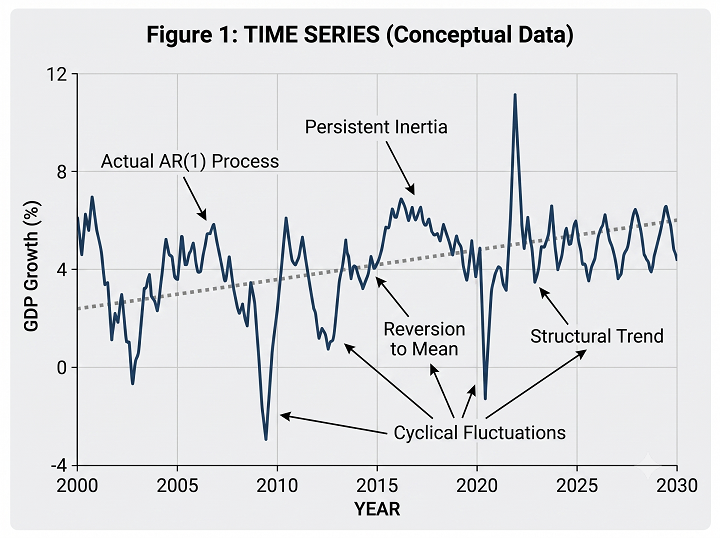
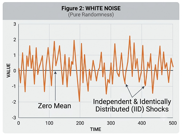
Understanding these patterns is the purpose of time-series analysis.

Among the classical tools, the AutoRegressive Moving Average (ARMA) model provides a foundational framework for describing how historical information propagates through time.

Although modern quantitative research employs far more sophisticated techniques, ARMA remains an essential starting point for understanding dynamic systems, forecasting, and statistical inference.

What Is a Time Series?

A time series is a sequence of observations indexed by time, such as daily stock returns, monthly inflation rates, annual productivity statistics, or personal income and consumption over time.

Unlike ordinary cross-sectional random data, time-series observations are inherently connected. A simple example is personal income and consumption. Income earned today influences tomorrow's spending, while accumulated experience and skills shape future productivity. Such observations are naturally connected over time rather than being independent.

The ordering of observations therefore contains valuable information.

Understanding these temporal relationships is the central objective of time-series modeling.

Autocorrelation: Does the Past Matter?

An intuitive question we can ask is:

Does a variable tend to resemble its own past values?

This concept is known as autocorrelation. Positive autocorrelation implies persistence: economic growth tends to continue, business cycles often evolve gradually; negative autocorrelation implies reversal: the economy may change direction, a successful business yesterday may become less competitive - or even obsolete - today. If no autocorrelation exists, observations behave like independent random shocks. Strong autocorrelation suggests that historical information still contains explanatory power for future outcomes.

Figure 3 Autocorrelation

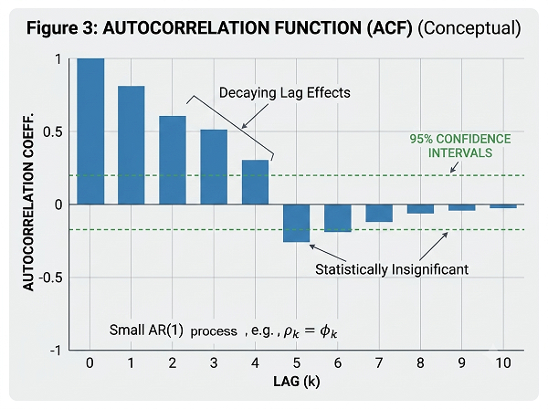
The purpose of autocorrelation function is to measure the statistical relationship between observations at different time lags. The autocorrelation coefficient at lag (k) measures the relationship between the current observation and its value (k) periods earlier.

The Autoregressive Moving Average (ARMA) model is a cornerstone of classical time-series analysis. Originally developed by Peter Whittle in 1951 and later popularized by George Box and Gwilym Jenkins through the Box--Jenkins methodology, ARMA models became one of the foundations of modern time-series analysis, providing a framework for understanding, representing, and forecasting the conditional mean of stationary stochastic process. I will introduce the AR, MA and their combination ARMA model in this article.

The Autoregressive Model (AR)

The Autoregressive (AR) model assumes that the present depends directly on previous observations.

An AR(1) process is expressed as:

$X_t = c + \phi_1 X_{t-1} + \epsilon_t$

Where $X_t$ denotes the value of the series at time $t$ , $c$ is a constant, $\phi_1$ is the coefficient that measures the influence of the previous observation $X_{t-1}$ on the current value, and $\epsilon_t$ represents a white-noise error term. This function expresses a simplified assumption:

Today's value equals a constant, plus a fraction of yesterday's value, plus a new random shock.

Figure 4 AR(1) Model

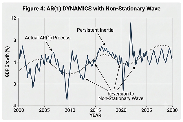
Examples include: Inflation persistence; Business cycles; Commodity prices, etc. The parameter $\phi$ measures memory: $\phi$ > 0 : persistence, $\phi$ < 0 : reversal, $\phi$ = 0 : no dependence. If the absolute value of coefficient exceeds 1, the process becomes unstable because shocks accumulate rather than dissipate. Therefore, a stationary AR(1) process requires $| \phi | < 1$ . In this way, many economic systems can be viewed as balancing persistence with adaptation.

The Moving Average Model (MA)

The Moving Average (MA) model approaches dynamics from another perspective.

Instead of depending on past observations themselves, it assumes that current values depend on past disturbances.

An MA(1) process is given by:

$y_t = \mu + \epsilon_t + \theta\epsilon_{t-1}$

The key idea is:

Economic systems remember shocks.

A large event---such as a policy announcement, technological breakthrough, or financial crisis---may influence behavior beyond the moment it occurs. The MA framework captures the lingering effects of these temporary disturbances.

In practice: Supply-chain disruptions affect future production, monetary policy announcements influence expectations for several periods, market surprises generate delayed responses from investors.

The parameter $\theta$ determines how strongly past shocks continue to shape present outcomes.

AR versus MA: Two Different Views of Dynamics

Although both models describe temporal dependence, their interpretations differ fundamentally.

Model	Interpretation	Economic Meaning
AR	Dependence on past values	Persistence and inertia
MA	Dependence on past shocks	Memory of disturbances
ARMA	Combination of both	Dynamic systems with inertia and shocks

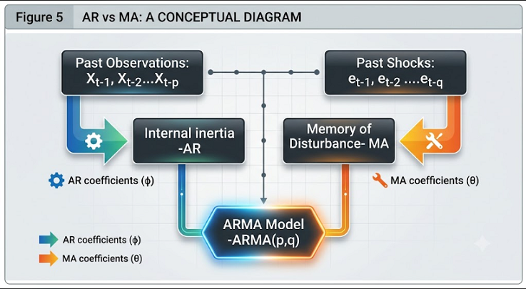
An AR model suggests that the system itself contains internal momentum.

An MA model suggests that the environment continuously injects shocks whose effects gradually dissipate.

Real-world systems often exhibit both characteristics simultaneously.

Figure 5 AR vs MA

The ARMA Model: Persistence Meets Innovation

The AutoRegressive Moving Average (ARMA) model combines these two mechanisms.

An ARMA(1,1) specification can be written as:

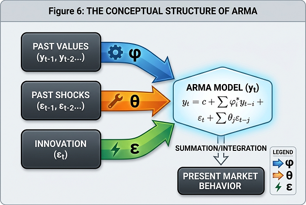
$y_t =c+\phi y_{t-1} + \epsilon_t + \theta\epsilon_{t-1}$

Conceptually, this means:

The present is shaped both by historical conditions and by memories of recent shocks.

Economic and financial systems rarely reset themselves each period. Organizations accumulate experience and transform it into knowledge assets and intellectual property. Consumers gradually update their expectations through repeated interactions with the market. Investors respond not only to current information but also to previous surprises. These dynamic interactions are exactly the type of behavior ARMA models seek to represent.

ARMA models provide a parsimonious framework for describing these interactions.

Figure 6 ARMA Model

Applications in Economics and Finance

ARMA models remain widely used in:

Macroeconomic Forecasting : GDP growth, Inflation, Unemployment, Industrial production.

Financial Analysis : Interest rates, Exchange rates, Commodity prices, Return processes.

Business Operations: Demand forecasting, Inventory management, Supply-chain planning, Energy consumption prediction.

Although many modern machine-learning approaches outperform classical methods in certain contexts, ARMA models possess important advantages:

Transparency.
Interpretability.
Statistical rigor.
Economic intuition.

Understanding them remains essential before moving toward more sophisticated frameworks.

Limitations of ARMA Models

Despite their usefulness, ARMA models face important limitations.

First, they assume relatively stable statistical structures over time.

Second, they primarily focus on the conditional mean rather than changing risk conditions.

Financial markets, however, exhibit a phenomenon known as volatility clustering:

Calm periods are followed by calm periods, and turbulent periods are followed by turbulence.

ARMA can describe expected dynamics, but it cannot adequately model evolving uncertainty.

This limitation motivates the development of the next generation of models:

ARCH (Autoregressive Conditional Heteroskedasticity)
GARCH (Generalized ARCH)

These frameworks shift attention from predicting returns to understanding risk itself. These models will be introduced in the following articles of this series.

Conclusion

Time-series analysis begins with a simple but profound question:

How much of the past survives into the present?

Autocorrelation provides the first clue. Autoregressive models capture persistence. Moving-average models describe the memory of shocks. ARMA integrates both mechanisms into a coherent framework for understanding dynamic systems.

For quantitative researchers, mastering these ideas is not merely a technical exercise. Rather than being merely a forecasting tool, ARMA provides a framework for thinking about how information, expectations, and shocks propagate through dynamic economic systems.

In the next article, we move from modeling expectations to modeling uncertainty itself, introducing the ARCH framework and the phenomenon of volatility clustering.