Understanding Financial Time Series Models (Part II): ARCH and Volatility Clustering

In the previous article, we introduced the ARMA model, which describes how historical information influences the expected behavior of a time series. In traditional time-series econometrics (like ARMA models), a core simplifying assumption is homoskedasticity---the assumption that the variance of the error term is constant over time.

However, empirical evidence from financial markets shows that asset returns rarely satisfy this assumption. Financial asset returns exhibit two well-known characteristics:

• Volatility clustering, where periods of high volatility are followed by high volatility and calm periods are followed by calm periods.

• Leptokurtosis (fat tails), where extreme price movements occur more frequently than predicted by the normal distribution.

To model this dynamic behavior, Robert Engle introduced the Autoregressive Conditional Heteroskedasticity (ARCH) model in 1982, a breakthrough that earned him the Nobel Prize in Economics in 2003.

Return measures the percentage change in an asset's price over a given period.

Volatility measures the variability or uncertainty of asset returns.

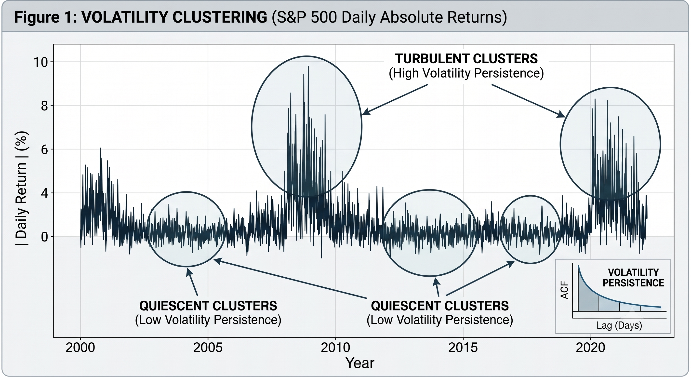
To explain these observations, we allow today's uncertainty to depend on yesterday's uncertainty. This idea leads to the ARCH model. Prior to ARCH, most econometric models assumed that uncertainty remained constant over time. Engle's key contribution was to recognize that volatility itself follows a dynamic process and can therefore be modeled and forecasted. This insight revolutionized financial econometrics and laid the foundation for modern volatility forecasting and financial risk management.

What is the ARCH Model

To understand the model, we can break down its name into its statistical components:

• Autoregressive: The current value of the variable is regressed on its own past (lagged) values. In this case, today's volatility is modeled as a function of past squared shocks.

• Conditional: The variance is not constant; it depends (is conditional) on the information available from the immediate past.

• Heteroskedasticity: The variance of the error terms is unequal, non-constant, and time-varying.

The standard ARCH(p) model decomposes a return series $r_t$ into a mean equation and a conditional variance equation. Let $p$ denote the number of lagged squared innovations ($\epsilon_{t - i}^{2}$) included in the conditional variance equation for calculating today's conditional variance. The return of an asset at time $t$ is modeled as:

$r_{t} = \mu_{t} + \epsilon_{t}$

$\mu_t$: The expected return which may be a constant $\mu$, an $AR(1)$ process, or even an $ARMA(p,q)$ process.

$\epsilon_t$: The residual or "shock" at time $t$.

The Error Term Decomposition

The shock $\epsilon_t$ is further decomposed to isolate its time-varying volatility:

$\epsilon_t = \sigma_t z_t$

$z_t$: A standardized, independent, and identically distributed (i.i.d.) random variable with mean $0$ and variance $1$ (typically assumed to follow a Standard Normal $\\mathcal{N}(0,1)$ or Student's $t$-distribution to capture fat tails).

$\sigma_t$: The conditional standard deviation (volatility) of the shock at time $t$.

The Conditional Variance Equation

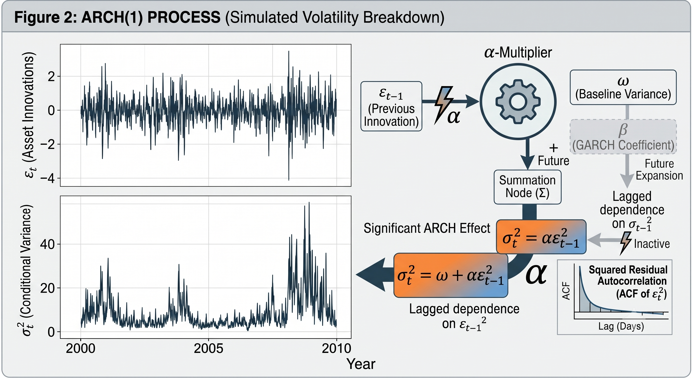
The core of the ARCH model is how it defines the conditional variance $\sigma_t^2$ as a weighted sum of past squared shocks:

$\sigma_t^2 = \alpha_0 + \alpha_1 \epsilon_{t-1}^2 + \alpha_2 \epsilon_{t-2}^2 + \dots + \alpha_p \epsilon_{t-p}^2$

Using summation notation:

$\sigma_{t}^{2} = \alpha_{0} + \sum_{\left\{ i = 1 \right\}}^{p}{\alpha_{i}\epsilon_{t - i}^{2}}$

Structural Constraints:

To ensure the model is physically and mathematically logical, we must apply strict boundaries to the parameters:

• Positive Variance: Variance cannot be negative. Therefore, we require:

• $\alpha_0 > 0 \quad \text{and} \quad \alpha_i \ge 0 \quad \text{for all } i = 1, \dots, p$

• Stationarity: For the variance process to be stable (and not explode to infinity), the sum of the lag coefficients must be strictly less than 1:

• $\sum_{i=1}^p \alpha_i < 1$

How the ARCH Model Works (Intuition)

ARCH suggests that markets learn from recent events. Today's uncertainty is influenced by the magnitude of yesterday's shocks. The variance equation represents a feedback loop:

• If a major economic event occurs yesterday (such as a market rush or crash), the residual $\epsilon\_{t-1}$ will be very large (positive or negative).

• Squaring this residual ($\epsilon\_{t-1}^2$) creates a massive positive input for today's variance equation.

• This causes today's conditional variance $\sigma_t^2$ to spike.

• Because $\sigma_t$ is high, the shock tomorrow ($\epsilon_t = \sigma_t z_t$) is likely to be large as well.

• This mathematical feedback loop replicates the real-world phenomenon of volatility clustering.

• Another important implication is leptokurtosis. Even if the underlying shocks $z_{t}$ follow a normal distribution, the return distribution generated by an ARCH process exhibits heavier tails than the normal distribution. This characteristic more closely resembles the behavior observed in real financial markets.

Practical Applications in Quantitative Finance

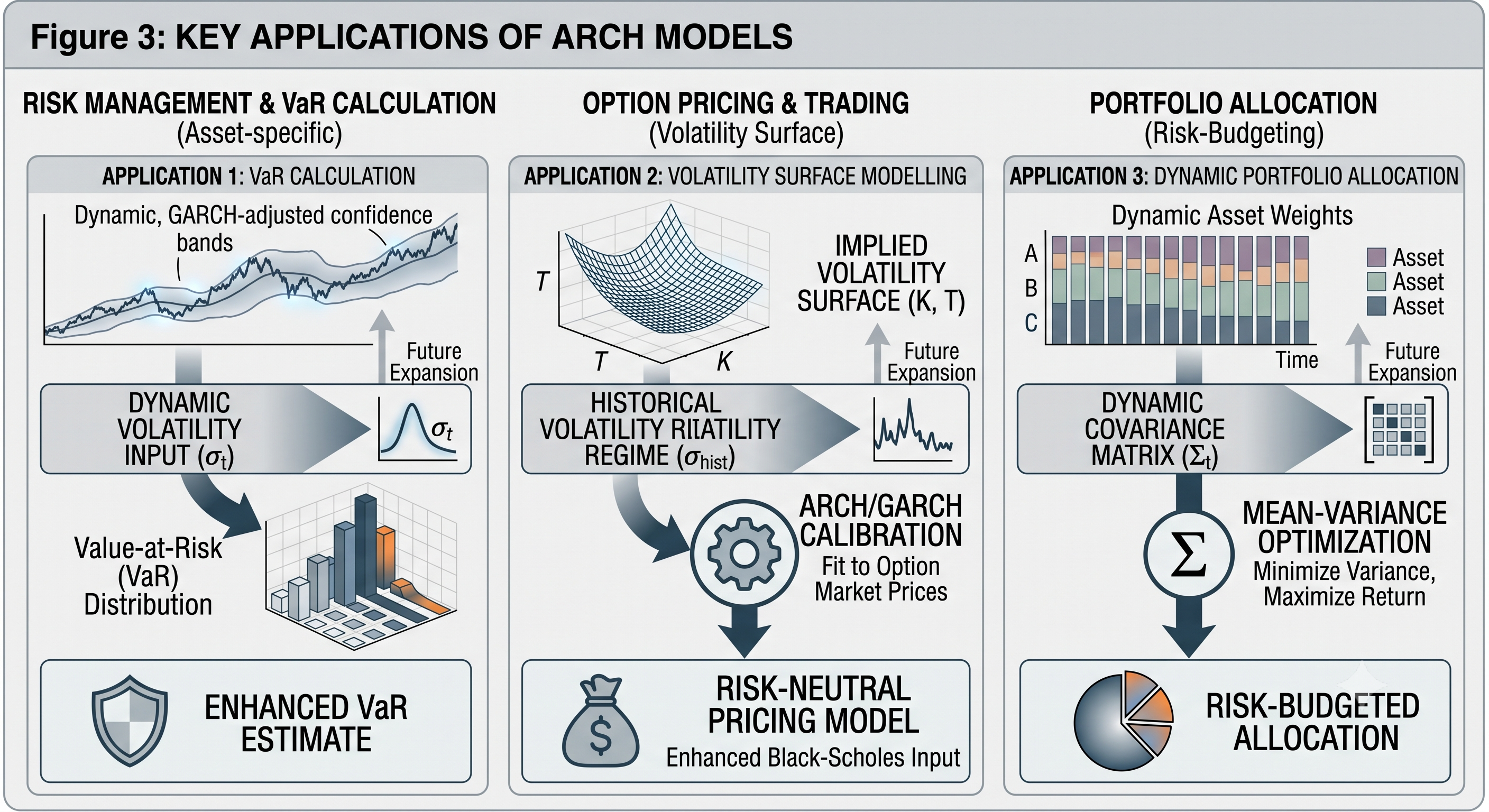
Dynamic Value at Risk (VaR) and CVaR

Unlike static historical VaR, an ARCH-based VaR dynamically widens its risk threshold during market corrections, preventing severe underestimation of downside risks. Since ARCH models place greater weight on recent shocks than on older shocks, the VaR floor spikes instantly on the day of a crash and decays smoothly and exponentially as the market calms down.

${\text{Dynamic~}\text{VaR}}_{t} = S_{t} \times \left( 1 - e^{- z_\alpha \sigma_{t}} \right)$

$S_{t}$: The current price of the stock or asset at time* $t$.

$\sigma_{t}$: The conditional standard deviation (volatility) of the daily log returns at time* $t$. It is "dynamic" because it updates daily, typically modeled via a rolling historical window, calculated directly from an ARCH($p$) variance equation.

$z_{\alpha}$: The critical value (z-score) from the standard normal distribution corresponding to the chosen confidence level* $\alpha$.

Option Pricing and the "Volatility Smile"

The Black-Scholes-Merton model assumes that volatility $\sigma$ is constant over the life of the option. In reality, implied volatility varies across different strike prices (the volatility smile) because market participants know volatility is stochastic.

• By using an ARCH framework to model the path of the underlying stock, option pricing models can simulate paths where volatility expands during market sell-offs, resulting in more accurate pricing for out-of-the-money options.

Asset Allocation and Portfolio Optimization

When constructing a multi-asset portfolio, the covariance matrix must be calculated. Standard covariance matrices are static. By applying multivariate ARCH models (such as CCC-GARCH or DCC-GARCH), portfolio managers can generate a dynamic covariance matrix that adjusts daily, helping them adjust asset allocations as market correlations evolve.

Limitations of ARCH and the Transition to GARCH

While revolutionary, the basic ARCH(p) model has a significant limitation:

• The Parameter Problem: Volatility in financial markets is highly persistent. To capture long-lasting volatility regimes, an ARCH(p) model often requires a very large number of lags (p). This means estimating many parameters ($\alpha_1, \alpha_2, \dots$), which introduces estimation error and reduces statistical power.

• Symmetry in Volatility Shocks: The model uses the squared past shock ($\epsilon_{t-i}^2$). Since positive and negative shocks become identical after squaring, the model cannot distinguish between good news and bad news. In reality, equity markets exhibit the leverage effect, where bad news triggers a much higher spike in panic and volatility than good news.

• No Direct Feedback on Asset Pricing: The basic ARCH model does not allow the expected return of an asset to depend directly on its current risk level, even though financial theory states that investors require a higher premium to hold riskier assets. (This was solved by the ARCH-M / ARCH-in-Mean extension).

Improved model: GARCH

To solve the parameter problem, Tim Bollerslev introduced the Generalized ARCH (GARCH) model in 1986. GARCH simplifies the equation by adding lagged conditional variance terms ($\sigma_{t-1}^2$) directly into the variance equation, mimicking an infinite-lag ARCH model with just a few parameters. GARCH model will be introduced in the next article.

SUMMARIZE

ARMA asks: How do past returns and shocks shape today's expected return?

ARCH asks: How does the past shocks influence today's uncertainty?

Instead of assuming constant risk, ARCH recognizes that financial markets alternate between calm and turbulent periods.

This insight fundamentally changed quantitative finance and laid the foundation for modern volatility forecasting, portfolio risk management, and derivative pricing.

In the next article, we will introduce GARCH, one of the most influential volatility models in financial economics, and explore why it remains one of the standard tools used by quantitative analysts, asset managers, and central banks today.

---