Understanding Financial Time Series Models (Part III): GARCH and Volatility Persistence

In the previous article, we introduced the Autoregressive Conditional Heteroskedasticity (ARCH) model, one of the most influential breakthroughs in modern financial econometrics. ARCH fundamentally changed the way economists and quantitative analysts think about financial risk by recognizing that volatility is not constant but evolves through time.

Instead of assuming a fixed level of uncertainty, ARCH allows today's risk to depend on yesterday's market shocks. This simple yet powerful idea successfully explains one of the most persistent empirical features of financial markets: volatility clustering.

Despite this breakthrough, ARCH has an important practical limitation.

Financial markets often exhibit long-lasting volatility persistence. After major events such as financial crises, monetary policy changes, or geopolitical conflicts, elevated market uncertainty may continue for weeks or even months. Capturing this behavior using a pure ARCH model requires incorporating a large number of lagged shocks, resulting in many parameters that are difficult to estimate and often lead to overfitting.

To address this problem, Tim Bollerslev introduced the Generalized Autoregressive Conditional Heteroskedasticity (GARCH) model in 1986.

By allowing current volatility to depend not only on previous shocks but also on previous volatility itself, GARCH provides a far more efficient representation of financial risk.

Today, GARCH remains one of the most influential models in financial economics and continues to serve as a standard tool for volatility forecasting, portfolio risk management, derivative pricing, stress testing, and quantitative investment research.

What is GARCH Model

Compared with the ARCH model, whose conditional volatility depends solely on past shocks, GARCH recognizes that volatility itself possesses inertia. Today's uncertainty depends not only on yesterday's unexpected market movements, but also on yesterday's level of uncertainty. As its names shows:

• Generalized: Expands the basic ARCH framework by adding lagged values of the conditional variance itself, dramatically reducing the number of parameters needed.

This seemingly small modification dramatically improved both statistical efficiency and forecasting performance. With only a few parameters, GARCH can reproduce the behavior of a very high-order ARCH model while providing more stable and accurate estimates of financial risk.

In GARCH model, the return of an asset at time $t$ is similar to ARCH:

$r_{t} = \mu_{t} + \epsilon_{t}$

$\mu_t$: The expected return which may be a constant $\mu$, an $AR(1)$ process, or even an $ARMA(p,q)$ process.

$\epsilon_t$: The residual or "shock" at time $t$.

The shock $\epsilon_t$ is further decomposed to isolate its time-varying volatility:

$\epsilon_t = \sigma_t z_t$

$z_t$: A standardized, independent, and identically distributed (i.i.d.) random variable with mean $0$ and variance $1$ (typically assumed to follow a Standard Normal $\mathcal{N}(0,1)$ or Student's $t$-distribution to capture fat tails).

$\sigma_t$: The conditional standard deviation (volatility) of the shock at time $t$.

The Conditional Variance Equation

The core of the GARCH model is how it defines the conditional variance $\sigma_t^2 = Var(r_t \mid \mathcal{F}_{t-1})$ is modeled as:

$\sigma_t^2 = \omega + \sum_{i=1}^{q} \alpha_i \epsilon_{t-i}^2 + \sum_{j=1}^{p} \beta_j \sigma_{t-j}^2$

$q$: The order of the ARCH terms (lags of past squared innovations $\epsilon_{t-i}^2$).

$p$: The order of the GARCH terms (lags of past conditional variances $\sigma_{t-j}^2$).

$\omega > 0$: The baseline constant variance floor.

$\alpha_i \ge 0$: Coefficients measuring the short-term impact of recent market shocks (ARCH parameters).

$\beta_j \ge 0$: Coefficients measuring the persistence/inertia of volatility (GARCH parameters).

Structural Constraints:

To ensure the model is physically and mathematically logical, we must apply strict boundaries to the parameters:

• Positive Variance: $\omega > 0, \alpha_i \ge 0, \beta_j \ge 0$ ensure that the calculated variance $\sigma_t^2$ is strictly positive for all $t$.

• Stationarity: For the variance process to be stable (and not explode to infinity), the sum of the lag coefficients must be strictly less than 1. For a general GARCH(p, q) model, stationarity requires:

$\sum_{i=1}^{q} \alpha_i + \sum_{j=1}^{p} \beta_j < 1$

• If $\alpha_1 + \beta_1 = 1$, the model becomes an Integrated GARCH (IGARCH) process, where shocks to volatility persist indefinitely (unit root in variance).

• If $\alpha_1 + \beta_1 > 1$, the conditional variance grows explosively over time.

How the GARCH Model Works (Intuition)

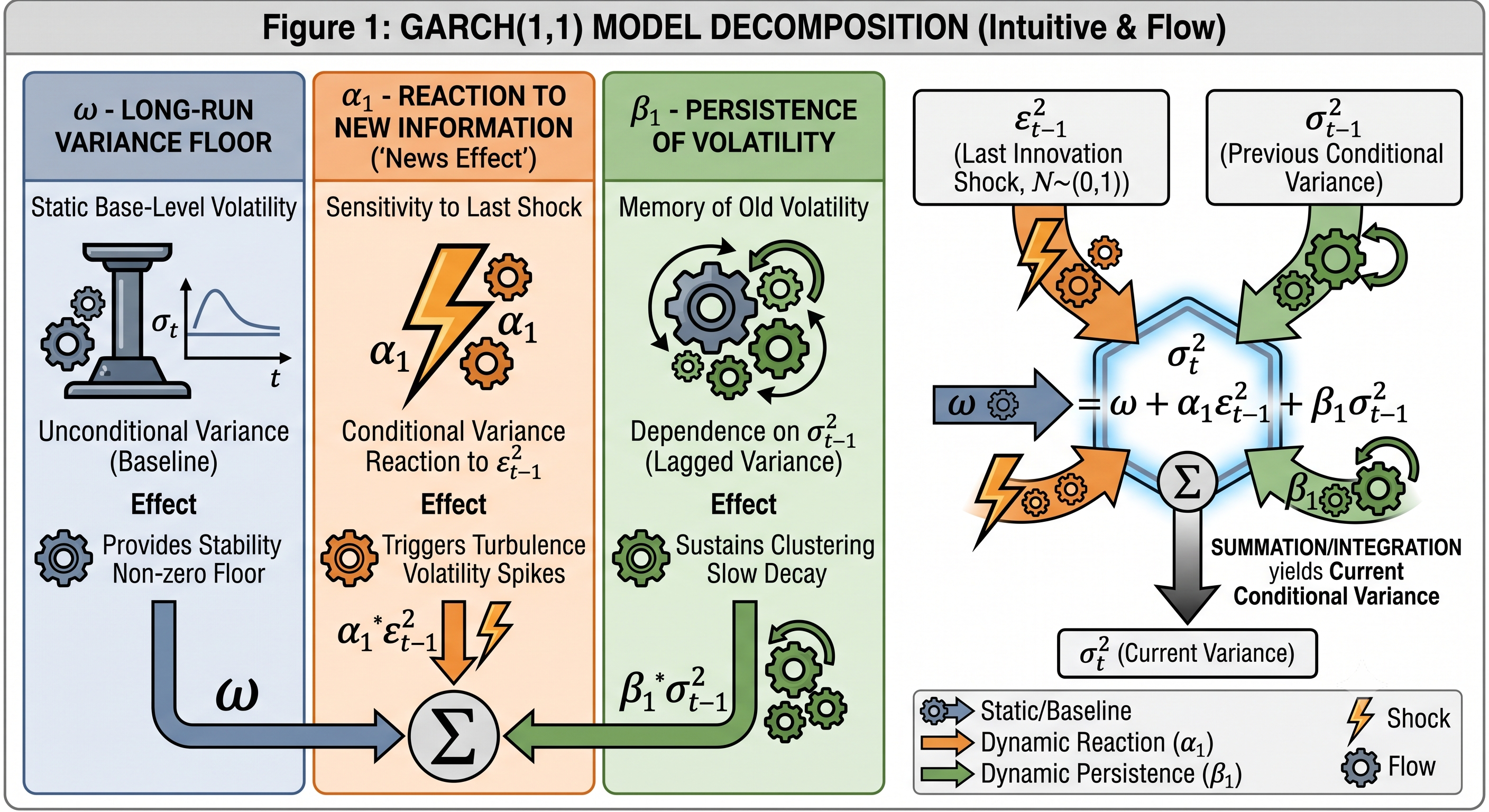
In empirical finance, high-order lag models are rarely necessary. The $GARCH(1, 1)$ model captures the vast majority of financial volatility dynamics using only three parameters:

$\sigma_t^2 = \omega + \alpha_1 \epsilon_{t-1}^2 + \beta_1 \sigma_{t-1}^2$

$\omega$ (Baseline Variance): The underlying long-term variance level to which the system decays in the absence of new shocks.

$\alpha_1$ (News Reaction Coefficient): Measures how strongly today's volatility reacts to an unexpected price move yesterday ($\epsilon_{t-1}^2$). A high $\alpha_1$ means volatility spikes aggressively following market shocks.

$\beta_1$ (Persistence Coefficient): Measures how long a volatility spike takes to dissipate. In daily asset returns, $\beta_1$ typically lies in the range of $0.80$ to $0.95$, reflecting strong volatility memory.

An $ARCH(q)$ model requires many lagged parameters ($q \> 10$) to capture persistent volatility, leading to over-parameterization and potential violations of positivity constraints. GARCH solves this parsimoniously.

A single $GARCH(1, 1)$ model is equivalent to an infinite-order $ARCH(\infty)$ model where the weights assigned to historical shocks decay geometrically at rate $\beta_1$.

Practical Applications in Quantitative Finance

Dynamic Value at Risk (VaR) and CVaR

Replaces static rolling-window standard deviations with a daily updated $\sigma_t$. This eliminates the "ghosting effect" of static windows and ensures risk thresholds dynamically expand during market crises.

$VaR_{t} = f\left( \sigma_{t} \right)$

This allows institutions to react much faster during market stress.

Option Pricing

The Black-Scholes-Merton model assumes that volatility $\sigma$ is constant over the life of the option. Real markets clearly violate this assumption. By generating realistic volatility paths, GARCH-based simulations improve pricing accuracy for equity options, commodity derivatives, and structured products.

Asset Allocation and Portfolio Optimization

When constructing a multi-asset portfolio, the covariance matrix must be calculated. Standard covariance matrices are static. GARCH allows portfolio risk to evolve through time, leading to dynamic asset allocation; adaptive leverage; risk budgeting; portfolio rebalancing.

Limitations of GARCH

Although GARCH became the industry standard, it still has several limitations. First, it has Symmetric Response. Positive and negative shocks influence volatility equally. In reality, bad news usually increases volatility much more than good news. This phenomenon is known as the Leverage Effect. Second, some financial assets exhibit persistence over years rather than months. Standard GARCH cannot fully capture these long-memory processes. Third, Financial markets may experience structural breaks, regime switching, or sudden crises. Linear GARCH models often struggle under these conditions.

To address these shortcomings, researchers proposed numerous extensions. Examples include EGARCH (Exponential GARCH), TGARCH / GJR-GARCH, FIGARCH, Multivariate GARCH, etc. Many of these remain active areas of quantitative finance research.

Summary

ARMA asks how do past returns and shocks shape today's expected return?

ARCH asks how do past shocks influence today's uncertainty?

GARCH asks How does uncertainty itself evolve over time?

Rather than treating volatility as an isolated reaction to recent events, GARCH recognizes that risk possesses persistence. This simple yet profound insight transformed financial econometrics. Nearly forty years after its introduction, GARCH remains one of the most important models used by quantitative analysts, hedge funds, investment banks, central banks, and academic researchers.

Understanding GARCH is therefore not merely learning another statistical model. It is learning one of the fundamental ways modern finance measures and manages uncertainty.

Looking Ahead

GARCH substantially improves ARCH by modeling persistent volatility with a parsimonious specification, making it one of the most influential models in modern financial econometrics.

However, forecasting volatility is only one part of risk management. Investors ultimately need to translate volatility forecasts into concrete measures of potential losses.

In the next article, we will introduce Value at Risk (VaR), one of the most widely used quantitative risk measures in finance, and explore how volatility models such as GARCH can be used to estimate portfolio downside risk.

---