Understanding Financial Time Series Models (Part IV): VaR/CVaR --- How Much Could We Lose?

Chen Quant Academy Series -- Introducing Quantitative Models in Finance

In the previous articles, we introduced three foundational time-series models:

ARMA --- how past observations and shocks shape expected returns;
ARCH --- how past shocks influence current volatility;
GARCH --- how volatility itself persists and evolves over time.

These models help us understand the dynamics of financial markets. But understanding volatility is not the same as understanding investment risk. An investor ultimately wants to know a much more practical question:

How much could I potentially lose?

This question leads to one of the most widely used risk measures in modern finance: Value at Risk (VaR). VaR does not attempt to predict exactly what tomorrow's return will be. Instead, it estimates a threshold for potential loss over a specified time horizon and confidence level.

In this sense, VaR represents an important transition from statistical modeling to practical risk management.

What Is Value at Risk?

At its core, Value at Risk answers a simple executive question:

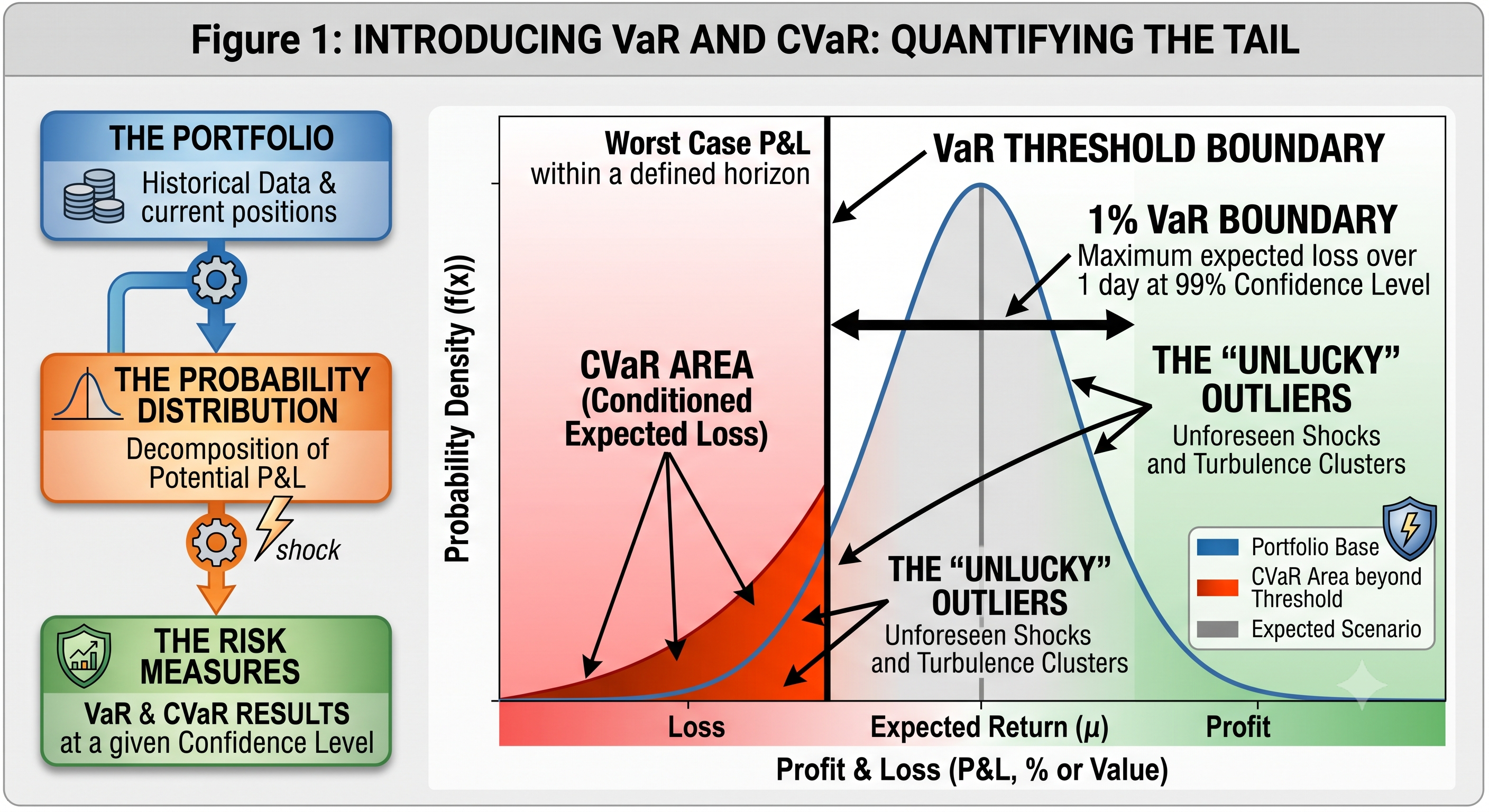
What is the loss threshold I should expect not to exceed over a given time horizon $T$ , at a specified confidence level $1-\alpha$ ?

It is a statistical measure that estimates the potential loss threshold of a portfolio over a specified time horizon at a given confidence level, under normal market conditions.

For example:

A one-day 95% VaR of $100,000 means that, under the model's assumptions, there is approximately a 5% probability that the portfolio will lose more than $100,000 over the next trading day.

The statement contains three important components:

VaR --- The threshold loss value in currency units or percent.
Time horizon T --- Over what period are we measuring the potential loss?
Confidence level $1-\alpha$ --- The statistical probability threshold (typically $95\%$ , $99\%$ , or $99.9\%$ ).

VaR as a Quantile of the Return Distribution

Suppose the portfolio return over the next period is represented by the random variable: $R\_{t+1}$ , The return distribution contains a range of possible outcomes. Most observations may be concentrated around the expected return, while extreme negative returns occupy the left tail of the distribution.

VaR focuses on the left tail of possible distribution. Importantly, in above example, a 99% VaR of $10000 does not mean that the maximum possible loss is $10,000. The portfolio can lose substantially more when events fall in the left tail part that exceed the threshold. Higher confidence does not mean higher certainty about the exact loss. It means we are moving further into the tail of the distribution.

Absolute VaR measures the loss threshold relative to zero wealth change (or initial investment); Relative VaR measures the loss threshold relative to the expected future portfolio value.

Figure 1 VaR and CVaR

Three Main Approaches to VaR

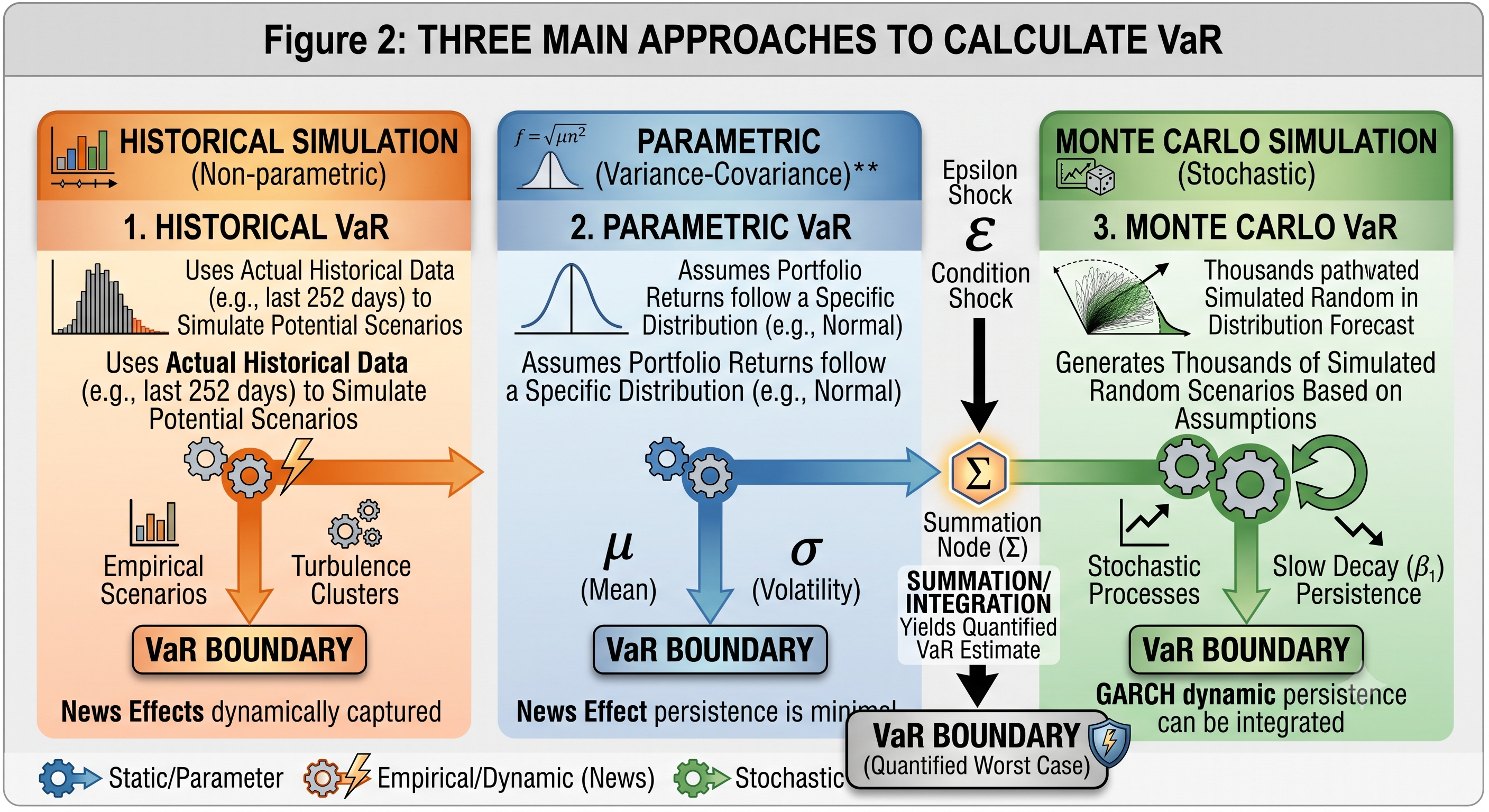
There are three classical approaches to estimating VaR:

Historical Simulation
Variance-Covariance / Parametric VaR
Monte Carlo Simulation

Each approach makes different assumptions about how the return distribution behaves.

1. Historical Simulation

The simplest approach is to use historical returns directly. Suppose we have 1,000 historical daily returns. We arrange them from the worst to the best: $R_{(1)}\le R_{(2)}\le \dots\le R_{(1000)}$ ，For a 95% VaR, we examine approximately the bottom 5% of observations.

The historical VaR is determined directly from the empirical distribution.

Historical simulation has an important advantage: It does not require us to assume that returns follow a particular probability distribution. This allows the historical sample to retain features such as skewness, fat tails, unusual market movements, non-normal return behavior.

However, the past may not represent the current market. A financial crisis that happened ten years ago may have little relevance to today's portfolio. Conversely, if a new crisis occurs that has never appeared in the historical sample, historical VaR may severely underestimate the risk.

Purely relying on historical sample data, historical VaR faces an important trade-off between historical information and current market conditions.

2. Parametric VaR

The second approach assumes a specific probability distribution for portfolio returns. The simplest example is the normal distribution. Suppose:

$R_{t+1}\sim N(\mu,\sigma^2)$

$\mu$ --- expected return;

$\sigma$ --- standard deviation, or volatility.

The VaR can then be expressed as:

$VaR_{1-\alpha} = -V_t(\mu+z_{\alpha}\sigma)$

$V_t$ is the portfolio value;

$\mu$ is the expected return;

$\sigma$ is the return volatility;

$z_{\alpha}$ <0 is the corresponding standard normal quantile in left tail.

If the expected return is relatively small compared with volatility, the equation is often approximated as:

$VaR_{1-\alpha}\approx V_t z_{1-\alpha}\sigma$

With the sign convention adjusted, $z_{\alpha}$ can be replaced by the equivalent positive quantile $z_{1-\alpha} = -z_{\alpha}$ .

Why GARCH Matters for VaR

This is where the previous articles become directly connected. A traditional parametric VaR model may assume that volatility is constant: $\sigma_t=\sigma$ , But financial markets clearly violate this assumption. As we discussed in the ARCH and GARCH articles, volatility changes over time.

GARCH provides an estimate of $\sigma_t$ that changes according to recent market shocks and previous volatility.

Therefore, instead of using a fixed volatility estimate, we can construct a conditional VaR based on $\sigma_t$ , Now the risk threshold changes with market conditions. When volatility rises, VaR rises; when volatility falls, VaR falls.

This creates an important connection between the models introduced throughout this series. While ARMA models expected returns, GARCH models conditional volatility, VaR translates these forecasts into a potential-loss threshold.

3. Monte Carlo VaR

Monte Carlo simulation takes a different approach.

Instead of relying only on historical observations, we specify a model for the behavior of the portfolio and generate a large number of simulated future scenarios. For example: $R_{t+1}^{(1)},R_{t+1}^{(2)},\dots, R_{t+1}^{(N)}$ . Each simulated return represents a possible future outcome.

After generating thousands or millions of scenarios, we construct the simulated return distribution and calculate the appropriate lower quantile. The resulting quantile provides the Monte Carlo VaR.

Monte Carlo methods are particularly useful for complex portfolios containing options, structured products, nonlinear positions, multiple risk factors. The trade-off is computational complexity. The more complicated the portfolio and model, the more scenarios may be required.

Concept Clarification for VaR and CVaR

VaR is not the maximum loss, but is a value at a threshold probability. It is intuitive to ask then: How large could those losses become once we are already beyond the VaR threshold? This leads to the next major risk measure: Expected Shortfall (ES), also known as Conditional Value at Risk (CVaR).

VaR identifies a threshold. Expected Shortfall asks what happens beyond that threshold. If the confidence level is 95%, Expected Shortfall measures the average loss among the worst 5% of outcomes.

$ES_{\alpha} = -E[R_t\mid R_t\le q_{1-\alpha}]$

$q_{1-\alpha}$ is the VaR return threshold;

$E[\cdot]$ represents the expected value;

the condition $R_t\le q_{1-\alpha}$ selects observations beyond the VaR threshold.

This provides information about the severity of tail losses that VaR alone cannot provide.

Figure 2 Three Approaches to VaR

VaR Backtesting

A VaR model is not useful simply because it produces a number. We need to test whether its predictions actually work. This process is known as backtesting.

Suppose we calculate a one-day 95% VaR every trading day. Over 1,000 trading days, we would expect approximately $1000\times(1-95%)=50$ exceptions, where the actual loss exceeds the predicted VaR. If the number of exceptions is dramatically higher than expected, the model may be underestimating risk. If there are far fewer exceptions than expected, the model may be excessively conservative.

Backtesting therefore provides an important feedback mechanism to allow risk models be tested against reality. This is particularly important because a sophisticated mathematical model itself doesn't guarantee correct estimations.

The Limitations of VaR

VaR is powerful, but it has several important limitations.

1. Model dependence

Different VaR methodologies can produce substantially different results. Historical VaR, parametric VaR, and Monte Carlo VaR may generate different estimates for exactly the same portfolio.

2. Tail blindness

VaR tells us where the tail begins, but not necessarily what happens after that point. This is why ES (CVaR) is often used alongside VaR.

3. Distribution assumptions

Parametric VaR often assumes a normal distribution. Financial returns, however, frequently exhibit fat tails, skewness, volatility clustering, regime changes. Therefore, a simple normal VaR model can underestimate extreme market risk.

4. Historical dependence

Historical simulation assumes that the past contains useful information about the future. That assumption is reasonable to some degree, but it can fail dramatically during unprecedented events.

5. Correlation instability

For multi-asset portfolios, VaR depends heavily on the relationships between assets. During market crises, correlations between assets can change rapidly. A portfolio that appears well diversified during normal periods may become highly concentrated in risk during a crisis.

From GARCH to VaR: Connecting the Models

At this point, the progression of the series becomes clearer.

ARMA: How do past returns and shocks shape today's expected return?

ARCH: How do past shocks influence today's uncertainty?

GARCH: How does uncertainty itself evolve over time?

VaR/CVaR: Given our estimate of the return distribution and volatility, how large could a loss become at/beyond a chosen confidence level?

This progression reflects an important development in quantitative finance. We begin with understanding the dynamics of returns, then model changing volatility, finally, we translate these statistical estimates into a practical risk-management measure.

Conclusion

Value at Risk represents an important bridge between quantitative modeling and practical financial risk management. It does not predict exactly what the market will do tomorrow. Instead, it provides a structured way to answer a more useful question: Given what we know about the market, what level of loss should we be prepared for?

Its power comes from combining probability, statistics, market data, and financial modeling. But VaR should never be treated as a guarantee. A risk model is only as useful as its assumptions, data, and validation.

This is why modern risk management rarely relies on a single number. VaR is typically combined with volatility models such as GARCH, stress testing, scenario analysis, and tail-risk measures such as CVaR.

The broader lesson is perhaps more important than the formula itself:

Quantitative risk management is not about predicting the future with certainty. It is about measuring uncertainty well enough to make better decisions.

Looking Ahead

VaR/CVaR provides a useful framework for translating probability distributions and volatility estimates into practical loss. However, quantitative finance is not only about measuring risk. It is also about understanding why different assets generate different returns.

In the next article, we will move from risk measurement to asset pricing and introduce the Fama--French Three-Factor Model, exploring how market risk, firm size, and value characteristics help explain differences in expected returns across stocks.

Author

Jia Chen

Master of Science in Software Development, Boston University
M.S. in Economics, Bocconi University
PMP®

Research interests:

Technology Innovation & Value Creation
Productivity & Organizational Management
Financial Markets & Quantitative Analysis
AI & Software Development

Chen Quant Center

https://www.chenquant.com

Chen Quant Center explores financial markets, quantitative models, data visualization, technology, and software-enabled research.